One of the central themes in ML over the past decade or so has been the convergence of modelling approaches, first across NLP tasks (translation, summarisation, question-answering), and then across modalities (NLP, vision, audio). Yes, the Transformer is everywhere. Increasingly though, we're just working with a specific variant of the original encoder-decoder: the decoder-only autoregressive (AR) model (GPT, Llama, etc.). Probably the biggest shift in the last year or two has been the increasing prevalence of the mixture-of-experts approach for the biggest of these models, but still we're mostly just working with AR decoding.

More recently though, people have started to revisit encoder-only architectures - the kind that were popular in the BERT era. One class of these are the Diffusion Language Models (Gemini Diffusion in particular caught my eye), and I think that these are worth keeping an eye on for several reasons:

• Diffusion has been the dominant paradigm in continuous domains like image generation for some time, which makes text diffusion an interesting alternate bridge towards genuinely multi-modal systems.
• There is also a potential latency advantage: unlike AR models that generate one token at a time, diffusion models can in principle generate a full sequence (or more realistically, a collection of subsequences) in parallel, enabling much faster generation.
• The generation process is also potentially more amenable to control and steering. For example, with standard AR models it can be quite tricky to reliably generate passages of specific lengths. For certain tasks, particularly those where in-filling matters, diffusion models (or at least, non-AR models) seem like a natural fit. In code generation, for example, you often have surrounding context that is fixed and just need to insert a new function, which is a more natural task for a bidirectional model than for an AR one.
• You can (again, in theory) correct errors during generation via iterative refinement.
• If you enjoy research (and I do), this is also just less of a well-trodden path at the moment, so there is potentially fun work to do here.

I had a vague idea of how diffusion worked in the continuous setting, so I decided to see how people were implementing diffusion LMs. Some of the math around diffusion can get quite dense, but the actual implementations turned out to be a lot simpler than I was expecting.

What are diffusion models?

Diffusion models have been around for a while [1], [2], [3], and others have already written nice explanations [4], [5], so I won't go into too much detail here. But at a high-level, diffusion models are a class of generative model, formed by first defining a procedure for turning data into noise over a sequence of steps, and then training a model to invert this process (and so map noise back into valid data). Of course these models are almost always some form of neural network, and as such you can expect usual suspects like the Transformer to show up again.

This process is described in Figure 1, taken from [3]. The function $q$ gradually transforms $\mathbf{x}_0$ into noise over $T$ steps, with each step conditioned on the previous step (forming a Markov chain).

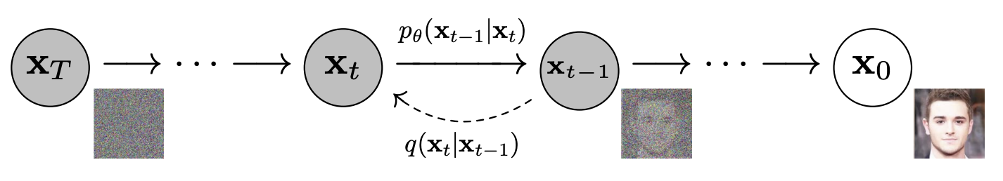
The goal is to learn $p_\theta$ to undo this process, and to do so we maximise a variational lower bound on the log-likelihood:

$$\mathbb{E} \left[ -\text{log} p_\theta(\mathbf{x}_0) \right] \leq \mathbb{E} \left[ -\text{log} \frac{p_\theta(\mathbf{x}_{0:T})}{q(\mathbf{x}_{1:T}|\mathbf{x}_0)} \right]$$

This decomposes into a sum of KL divergence terms [3]:

$$\mathbb{E}_q\left[ D_\text{KL}(q(\mathbf{x}_T|\mathbf{x}_0) \| p(\mathbf{x}_T)) + \sum_{t=2}^{T} D_\text{KL}(q(\mathbf{x}_{t-1}|\mathbf{x}_t, \mathbf{x}_0) \| p_\theta(\mathbf{x}_{t-1}|\mathbf{x}_t)) - \log p_\theta(\mathbf{x}_0|\mathbf{x}_1) \right]$$

The first term is a fixed prior matching term (no learnable parameters), and the last term $-\log p_\theta(\mathbf{x}_0|\mathbf{x}_1)$ is a reconstruction term: it measures how well the model can recover the original clean data from $\mathbf{x}_1$, the data corrupted with the smallest amount of noise.

In the middle term each $q(\mathbf{x}_{t-1}|\mathbf{x}_t, \mathbf{x}_0)$ is tractable (it's Gaussian in this case), so each KL can be computed in closed form. Because the forward process is Gaussian, $\mathbf{x}_t$ can be sampled directly from $\mathbf{x}_0$ in one step as $\mathbf{x}_t = \sqrt{\bar{\alpha}_t}\,\mathbf{x}_0 + \sqrt{1 - \bar{\alpha}_t}\,\boldsymbol{\epsilon}$, where $\boldsymbol{\epsilon} \sim \mathcal{N}(\mathbf{0}, \mathbf{I})$ and $\bar{\alpha}_t$ is the product of noise schedule terms. Reparameterising so that the model predicts the noise $\boldsymbol{\epsilon}$ rather than $\mathbf{x}_{t-1}$ directly (and dropping a weighting term), the training objective becomes:

$$\mathbb{E}_{t,\,\mathbf{x}_0,\,\boldsymbol{\epsilon}}\left[\|\boldsymbol{\epsilon} - \boldsymbol{\epsilon}_\theta(\mathbf{x}_t, t)\|^2\right]$$

So, you can sample a random $t$, corrupt the data with the corresponding amount of Gaussian noise, and train the model to predict that noise.

Text diffusion

This is all well and good for continuous domains such as vision and audio, but how does this apply to the discrete sequences of tokens that we currently use for text? In general, we have two options:

1. Map the discrete sequences into some continuous space first, then do diffusion in that space.
2. Use some sort of discrete diffusion process instead.

Both approaches are active areas of research at the moment; the jury is still out somewhat on which will ultimately prove the most fruitful. Here though I'm going to focus on discrete diffusion, specifically by using masking noise, which also makes the connection back to models like BERT more salient.

We're going to look at Simple and Effective Masked Diffusion Language Models [6], and as the name suggests, the core of the method is quite straight-forward. However, the actual code that was released for the paper is quite hard to read in my opinion (and tangled up with a lot of other approaches and baselines that they compare to), so it can be quite hard to figure out exactly what is going on. In this post I'm going to break it down, starting here with an overview of the method, then looking at a simple reimplementation.

Figure 2 gives an overview of the Masked Diffusion Language Model (MDLM) from [6]:

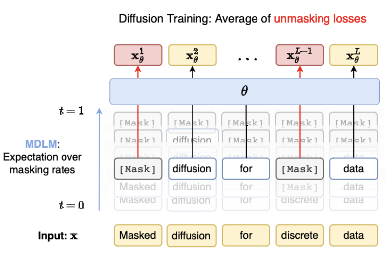
The training objective is a variant of the ELBO, and in their continuous-time formulation it simplifies to a reweighted cross-entropy over masked positions:

$$\mathbb{E}_{t \sim \mathcal{U}[0,1],\mathbf{x}_t \sim q(\cdot|\mathbf{x}_0)}\left[\frac{\alpha'_t}{1-\alpha_t}\sum_{\ell} \log p_\theta(x_0^\ell \mid \mathbf{x}_t)\right]$$

where $\alpha_t$ is a strictly decreasing noise schedule ($\alpha_0 \approx 1$, $\alpha_1 \approx 0$), $\ell$ is the sequence index, and the sum is implicitly weighted by whether the token at position $\ell$ is masked or not (unmasked tokens cannot contribute to the loss).

The training loop is therefore quite straight-forward:

• Sample $t$
• Generate the appropriate mask
• Run the model and then compute the weighted cross-entropy on the masked positions

There are a few small implementation details that we'll look at below, but in general the training setup ends up being quite close to the BERT-style masked language model. The main difference is that instead of the fixed masking rate that BERT was trained with, there is now a random masking rate during training (and the loss for each step is weighted depending on this masking rate). There is also the question of how to do generation using these models, which we will also look at in the next section.

A minimal implementation of masked diffusion language models

I have created a simple reimplementation of the MDLM code at github.com/johnglover/text-diffusion. It's not scaleable, but is hopefully useful as a learning resource. In the following sections I will walk through some of the most important parts of the training and generation code paths.

Model

The model architecture is one area where I deviate substantially from the MDLM paper. The authors use the transformer implementation from [8], which in turn is based on the diffusion transformer [9]. Instead, I am using the GPT2 implementation from Nanochat, as I want to compare AR and diffusion with as few changes as possible (more on this later). GPT2 here is a causal (decoder-only) LM, so the main change that I make is that I replace the causal attention with a full bidirectional attention. Apart from that, it's pretty much a standard modern transformer with the following features: RoPE positional embeddings, QK normalization, untied weights for token embedding and LM head, and functional RMSNorm (no learnable parameters). In the Nanochat experiments below, I use the 24-layer version of this model.

You can view the code at https://github.com/johnglover/text-diffusion/blob/main/src/text_diffusion/gpt2.py.

Training

Running train.sh starts the training loop in train.py, the code around line 50 is as follows:

# ... before: setup opt, dataloaders, etc.

for batch in dataloader:
    x = batch["input_ids"].to(device)
    attention_mask = batch["attention_mask"].to(device)
    batch_size = x.shape[0]

    t = sample_t(batch_size, device)
    sigma, dsigma = log_linear_noise(t)
    mask_prob = 1 - torch.exp(-sigma[:, None])

    x_masked = mask(x, mask_prob, tokenizer.mask_token_id)
    logits = model(x_masked)

    loss = diffusion_loss(
        logits,
        x,
        x_masked,
        tokenizer.mask_token_id,
        attention_mask,
        sigma,
        dsigma,
    )
    loss = loss.sum() / attention_mask.sum()

sample_t gets a batch of random timestamp samples. Conceptually we'd like to just do something like torch.rand(batch_size), but instead we draw the samples using a variance reduction technique called stratified sampling:

def sample_t(n, device="cpu"):
    sampling_eps = 1e-3
    eps_t = torch.rand(n, device=device)
    offset = torch.arange(n, device=device) / n
    eps_t = (eps_t / n + offset) % 1
    return (1 - sampling_eps) * eps_t + sampling_eps

Here, the unit interval [0, 1] is divided into n equal sub-intervals: [0, 1/n, 2/n, ..., (n-1)/n], then random jitter is added within each bin. The modulo makes sure that these values stay in [0, 1). This function basically just ensures samples are more evenly distributed across [0, 1] rather than purely random. This gives better coverage of the time dimension in diffusion training, leading to more stable gradients and better training dynamics.

Now that we have the sampled timestep $t$, we use it to compute the actual noise level for this step, according to some noise schedule.

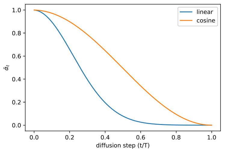
In our MDLM implementation, we're using their log-linear noise schedule, computed as follows:

def log_linear_noise(t, eps=1e-3):
    total = -torch.log1p(-(1 - eps) * t)
    rate = (1 - eps) / (1 - (1 - eps) * t)
    return total, rate

As the masking probability is $1 - e^{-\sigma}$, this will result in a masking rate that is linear in $t$: $(1-\epsilon) \cdot t$. This will in turn spread the masking probability evenly across time, or in other words, each time step unmasks roughly the same number of tokens. This is probably intuitively what you would guess should happen, but is worth mentioning here as there are other potential strategies (eg: unmask more or less at higher noise levels, etc.).

The function returns both the total noise level and the derivative at time $t$, as both are needed to weight the loss term later.

Given the total noise at $t$ we get the masking rate, then call our mask function, that replaces the corresponding percentage of input tokens x with the tokenizer.mask_token_id:

def mask(x, mask_prob, mask_token_id):
    mask_indices = torch.rand(*x.shape, device=x.device) < mask_prob
    return torch.where(mask_indices, mask_token_id, x)

The masked tokens are then used in the model forward pass to get our predictions:

x_masked = mask(x, mask_prob, tokenizer.mask_token_id)
logits = model(x_masked)

Finally, we compute our diffusion loss, before doing the usual backprop steps:

def subs(logits, x_masked, mask_token_id):
    """
    MDLM "SUBS" parameterisation
    """
    inf = 1e6

    # log prob at the mask token id = -infinity
    logits[:, :, mask_token_id] = -inf

    # normalize so x.exp() is a probability distribution over vocab_size
    logits = logits - torch.logsumexp(logits, dim=-1, keepdim=True)

    # For unmasked positions, create delta distributions:
    # Set probability = 1 for the observed token, 0 for all others.
    # This implements "carry-over unmasking" where unmasked tokens
    # are deterministically copied through.
    unmasked = x_masked != mask_token_id
    logits[unmasked] = -inf
    logits[unmasked, x_masked[unmasked]] = 0

    return logits


def diffusion_loss(
    logits, x, x_masked, mask_token_id, attention_mask, sigma, dsigma
):
    logits = subs(logits, x_masked, mask_token_id)
    log_p_theta = torch.gather(
        input=logits, dim=-1, index=x[:, :, None]
    ).squeeze(-1)
    loss = -log_p_theta * (dsigma / torch.expm1(sigma))[:, None]
    loss *= attention_mask
    return loss

In comparison to the usual cross-entropy over missing tokens, there are a couple of extra operations here:

1. Following the MDLM SUBS parameterisation, we make sure that unmasked tokens do not contribute to the loss.
2. The log probabilities are weighted by the noise level for the timestep: (dsigma / torch.expm1(sigma)).

That's it for the training loop, everything else is as you might expect if training an autoregressive model.

Generation

Similarly to training, our generation flow starts with generate.py (see a run example in generate.sh).

After loading our dependencies, the main generation function looks like this (slightly simplified):

def generate(model, tokenizer, config, device="cpu"):
    eps = 1e-5
    batch_size = config.batch_size
    N = config.gen_diffusion_steps

    x = tokenizer.mask_token_id * torch.ones(
        (batch_size, config.max_length),
        dtype=torch.int64,
        device=model.device,
    )

    timesteps = torch.linspace(1, eps, N + 1, device=model.device)
    dt = (1 - eps) / N

    for i in tqdm(range(N)):
        t = timesteps[i] * torch.ones(x.shape[0], 1, device=model.device)
        x = denoise_step(model, x, t, dt, tokenizer.mask_token_id)

    # final noise removal, in case some tokens are still masked
    logits = model(x)
    x = subs(logits, x, tokenizer.mask_token_id).argmax(dim=-1)

    return tokenizer.batch_decode(x)

We create an initial vector of (batch_size, max_length) mask tokens, that will ultimately be populated with our output tokens by the model. We also create our timesteps, uniformly spaced from $1$ down to $\epsilon \approx 0$ in $N + 1$ points. For each timestep, we perform one denoising step using the output from the previous step as the new input. At the end, we perform a final denoising step in case some tokens are still masked, and return the detokenized text.

Taking a slightly closer look at the denoise_step:

def denoise_step(model, x, t, dt, mask_token_id):
    s = t - dt

    logits = model(x)
    p = subs(logits, x, mask_token_id).exp()

    t = t[:, :, None]
    s = s[:, :, None]
    assert t.ndim == p.ndim

    q = p * (t - s)
    q[:, :, mask_token_id] = s[:, :, 0]
    samples = sample_categorical(q)

    unmasked = (x != mask_token_id).to(x.dtype)
    return (unmasked * x) + ((1 - unmasked) * samples)

denoise_step takes the sequence at noise level $t$ and produces a slightly less noisy version at $s = t - \Delta t$. First, the model runs a forward pass on the current (partially masked) sequence, then we apply the SUBS parameterisation to get the probability p over the vocabulary for each position. For unmasked positions this is a delta distribution on the observed token, and for masked positions it's the model prediction. We then create q from which we'll actually sample.

For each masked position, q has two outcomes:

1. Unmask: with probability proportional to $p \cdot (t - s)$ (the model's predicted probability scaled by the step size).
2. Remain masked: with probability proportional to $s$ (the current noise level).

The fraction of tokens unmasked at each step is proportional to $\Delta t / t$, the fraction of the remaining time interval being consumed. As $t$ gets closer to zero, fewer tokens remain masked, and the probability of staying masked decreases. Finally, tokens that were already unmasked are carried forward unchanged.

def sample_categorical(categorical_probs):
    gumbel_norm = 1e-10 - (torch.rand_like(categorical_probs) + 1e-10).log()
    return (categorical_probs / gumbel_norm).argmax(dim=-1)

sample_categorical performs the sampling using the Gumbel-max trick: rather than the standard approach of normalising q with a softmax then calling a multinomial sampler, we divide the probabilities by exponentiated Gumbel noise and take the argmax. This is mathematically equivalent, often more numerically stable, and faster in this instance at least according to my benchmarking.

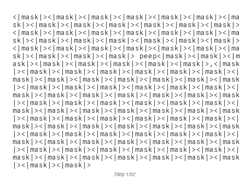
That's it for the generation loop. We can use these steps together to train small models. For example, Figure 4 shows the output from a training sanity check where I deliberately overfit on the opening 128 tokens from Alice in Wonderland. Here we generate 128 tokens over 32 steps (so 4 per step in parallel).

I haven't discussed any serious evaluation here, but we'll correct that in the next section, where I see if I can scale this up a bit.

Nanochat diffusion

To see how this works at a slightly larger scale, I ported this code to be usable as a drop-in replacement for pretraining in Andrej Karpathy's Nanochat repo. For those who are unaware, Nanochat is a relatively simple test bed for training LLMs (typically up to about GPT2 size). The idea is to cover the main stages (tokenisation, pretraining, finetuning, eval, inference) but keep things hackable.

I won't walk through the necessary repo changes in detail, but it's very close to my simplified version in my text-diffusion codebase that is described above, with just a few extra bits and pieces that were needed to integrate with the Nanochat setup. You can view the changes by comparing my diffusion branch where this code lives to the master branch.

Instead, we'll just look at some evaluations.

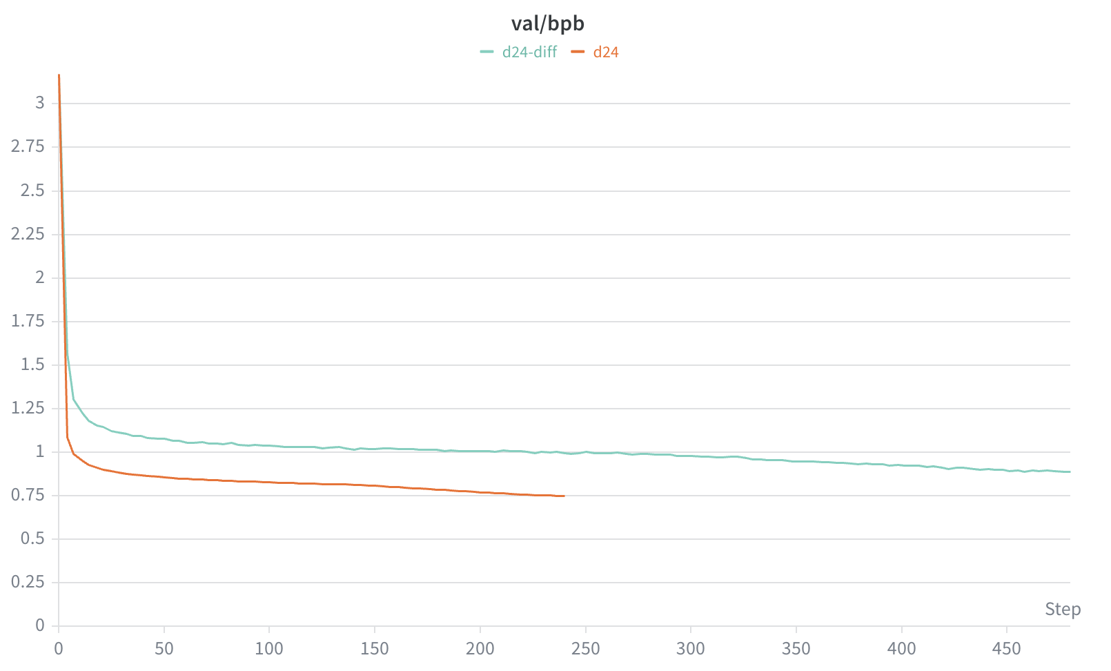
First, we note one obvious downside to diffusion LMs: training is much less efficient than with AR models. This should seem somewhat intuitive - for a given sequence, an AR model will predict every token, and so receive learning signal for every token in the sequence. Diffusion LMs on the other hand, will randomly be masking some percentage of tokens in the sequence every time we process it, and so on average (depending on noise schedules) will typically only actually be predicting roughly half the tokens in the sequence. So to get to a fair comparison in terms of number of predictions during training, we need to train on double the amount of tokens.

Looking at the validation curves over time, we do indeed see that we need to look at considerably more tokens before the diffusion LM perplexity gets even close to where the AR model is (and even at that, we're not quite getting there):

How do these perplexity values reflect downstream performance?

Task	Autoregressive	Diffusion
hellaswag_zeroshot	0.346	0.173
jeopardy	0.159	0.062
bigbench_qa_wikidata	0.522	0.414
arc_easy	0.563	0.469
arc_challenge	0.182	0.104
copa	0.380	0.100
commonsense_qa	0.044	0.083
piqa	0.418	0.312
openbook_qa	0.176	0.045
lambada_openai	0.433	0.268
hellaswag	0.349	0.232
winograd	0.370	0.077
winogrande	0.160	-0.040
bigbench_dyck_languages	0.109	0.160
agi_eval_lsat_ar	0.076	0.044
bigbench_cs_algorithms	0.405	0.434
bigbench_operators	0.171	0.129
bigbench_repeat_copy_logic	0.031	0.063
squad	0.354	0.454
coqa	0.257	0.264
boolq	-0.239	0.063
bigbench_language_identification	0.178	0.151
CORE	0.248	0.185

Quite accurately, it seems, when we look at the nanochat CORE evals. The AR model is better on 15 of 22 tasks (and CORE overall), with diffusion being ahead on the remaining 7 tasks. It is interesting to see where the bigger differences are; the diffusion model is noticeably ahead on squad, and behind on winograd and copa.

I did the pretraining run for this project a couple of months ago, so my branch is a bit behind now, it might be interesting to update and run these numbers again. We could also use something like autoresearch to try to improve this. But of course, these are just the zero-shot pretraining evals, for real use we would need to see what happens when we apply further training stages to the diffusion models (instruction tuning, RLHF, etc.).

Closing thoughts

On this simple pretraining and eval setup, AR models are better on most tasks and more efficient to train. But, there are a few tasks where the diffusion model is ahead in a way that seems potentially meaningful rather than noise. Whether that holds at scale, and whether the training efficiency story improves as more research is done on these types of models is something to keep an eye on. In any case however, the pretraining evals at GPT-2 scale are a noisy signal for real-world usefulness, and the structural differences between AR and diffusion models seem likely to matter more when we get to instruction tuning and RLHF.

Overall though this was a fun exercise. For people like me who have been mostly higher up the LLM stack in the world of post-training for the past few years, it was a good reminder that it is now relatively easy for individuals to pretrain something like GPT2 on a single machine in a few hours. And as for diffusion LMs - the basic code can be very straight-forward, there is genuinely interesting open work here, and it doesn't require a large team or a large budget to start experimenting.

References

[1]: Deep Unsupervised Learning using Nonequilibrium Thermodynamics

[2]: Generative Modeling by Estimating Gradients of the Data Distribution

[3]: Denoising Diffusion Probabilistic Models

[4]: https://lilianweng.github.io/posts/2021-07-11-diffusion-models

[5]: https://spacehunterinf.github.io/blog/2025/diffusion-language-models

[6]: Simple and Effective Masked Diffusion Language Models

[7]: Improved Denoising Diffusion Probabilistic Models

[8]: Discrete Diffusion Modeling by Estimating the Ratios of the Data Distribution

[9]: Scalable Diffusion Models with Transformers