Originally published on Aylien's blog.
I presented some preliminary work on using Generative Adversarial Networks to learn distributed representations of documents at the recent NIPS workshop on Adversarial Training. In this post I provide a brief overview of the paper and walk through some of the code.
Learning document representations
Representation learning has been a hot topic in recent years, in part driven by the desire to apply the impressive results of Deep Learning models on supervised tasks to the areas of unsupervised learning and transfer learning. There are a large variety of approaches to representation learning in general, but the basic idea is to learn some set of features from data, and then using these features for some other task where you may only have a small number of labelled examples (such as classification). The features are typically learned by trying to predict various properties of the underlying data distribution, or by using the data to solve a separate (possibly unrelated) task for which we do have a large number of labelled examples. This ability to do this is desirable for several reasons. In many domains there may be an abundance of unlabelled data available to us, while supervised data is difficult and/or costly to acquire. Some people also feel that we will never be able to build more generally intelligent machines using purely supervised learning (a viewpoint that is illustrated by the now infamous LeCun cake slide). Word (and character) embeddings have become a standard component of Deep Learning models for natural language processing, but there is less consensus around how to learn representations of sentences or entire documents. One of the most established techniques for learning unsupervised document representations from the literature is Latent Dirichlet Allocation (LDA). Later neural approaches to modeling documents have been shown to outperform LDA when evaluated on small news corpus (discussed below). The first of these is the Replicated Softmax, which is based on the Restricted Boltzmann Machine, and then later this was also surpassed by a neural autoregressive model called DocNADE. In addition to autoregressive models like the NADE family, there are two other popular approaches to building generative models at the moment - Variational Autoencoders and Generative Adversarial Networks (GANs). This work is an early exploration to see if GANs can be used to learn document representations in an unsupervised setting.
Modeling Documents with Generative Adversarial Networks
In the original GAN setup, a generator network learns to map samples from a (typically low-dimensional) noise distribution into the data space, and a second network called the discriminator learns to distinguish between real data samples and fake generated samples. The generator is trained to fool the discriminator, with the intended goal being a state where the generator has learned to create samples that are representative of the underlying data distribution, and the discriminator is unsure whether it is looking at real or fake samples. There are a couple of questions to address if we want to use this sort of technique to model documents:
- At Aylien we are primarily interested in using the learned representations for new tasks, rather than doing some sort of text generation. Therefore we need some way to map from a document to a latent space. One shortcoming with this GAN approach is that there is no explicit way to do this - you cannot go from the data space back into the low-dimensional latent space. So what is our representation?
- As this requires that both steps are end-to-end differentiable, how do we represent collections of discrete symbols?
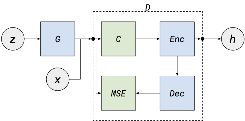
To answer the first question, some extensions to standard GAN model train an additional neural network to perform this mapping (like this, this and this). Another more simple idea is to just use some internal part of the discriminator as the representation (as is done in the DCGAN paper). We experimented with both approaches, but so far have gotten better results with the latter. Specifically, we use a variation on the Energy-based GAN model, where our discriminator is a denoising autoencoder, and use the autoencoder bottleneck as our representation (see the paper for more details). As for representing discrete symbols, we take the most overly-simplified approach that we can - assume that a document is just a binary vector of bag-of-words (ie, a vector in which there is a 1 if a given word in a fixed vocabulary is present in a document, and a 0 otherwise). Although this is actually still a discrete vector, we can now just treat it as if all elements are continuous in the range [0, 1] and backpropagate through the full network. The full model looks like this:

Here $z$ is a noise vector, which passes through a generator network $G$ and produces a vector that is the size of the vocabulary. We then pass either this generated vector or a sampled bag-of-words vector from the data ($x$) to our denoising autoencoder discriminator $D$. The vector is then corrupted with masking noise $C$, mapped into a lower-dimensional space by an encoder, mapped back to the data space by a decoder and then finally the loss is taken as the mean-squared error between the input to $D$ and the reconstruction. We can also extract the encoded representation ($h$) for any input document.
An overview of the TensorFlow code
The full source for this model can be found at https://github.com/johnglover/adversarial-document-model, here will just highlight some of the more important parts. In TensorFlow, the generator is written as:
def generator(z, size, output_size):
    h0 = tf.nn.relu(slim.batch_norm(linear(z, size, 'h0')))
    h1 = tf.nn.relu(slim.batch_norm(linear(h0, size, 'h1')))
    return tf.nn.sigmoid(linear(h1, output_size, 'h2'))
This function takes parameters containing the noise vector z, the size of the generator’s hidden dimension and the size of the final output dimension. It then passes noise vector through two fully-connected RELU layers (with batch norm), before passing the output through a final sigmoid layer. The discriminator is similarly straight-forward:
def discriminator(x, mask, size):
    noisy_input = x * mask
    h0 = leaky_relu(linear(noisy_input, size, 'h0'))
    h1 = linear(h0, x.get_shape()[1], 'h1')
    diff = x - h1
    return tf.reduce_mean(tf.reduce_sum(diff * diff, 1)), h0
It takes a vector x, a noise vector mask and the size of the autoencoder bottleneck. The noise is applied to the input vector, before it is passed through a single leaky RELU layer and then mapped linearly back to the input space. It returns both the reconstruction loss and the bottleneck tensor. The full model is:
with tf.variable_scope('generator'):
    self.generator = generator(z, params.g_dim, params.vocab_size)

    with tf.variable_scope('discriminator'):
        self.d_loss, self.rep = discriminator(x, mask, params.z_dim)

    with tf.variable_scope('discriminator', reuse=True):
        self.g_loss, _ = discriminator(self.generator, mask, params.z_dim)

    margin = params.vocab_size // 20
    self.d_loss += tf.maximum(0.0, margin - self.g_loss)

    vars = tf.trainable_variables()
    self.d_params = [v for v in vars if v.name.startswith('discriminator')]
    self.g_params = [v for v in vars if v.name.startswith('generator')]

    step = tf.Variable(0, trainable=False)

    self.d_opt = tf.train.AdamOptimizer(
        learning_rate=params.learning_rate,
        beta1=0.5
    )

    self.g_opt = tf.train.AdamOptimizer(
        learning_rate=params.learning_rate,
        beta1=0.5
    )
We first create the generator, then two copies of the discriminator network (one taking real samples as input, and one taking generated samples). We then complete the discriminator loss by adding the cost from the generated samples (with an energy margin), and create separate Adam optimisers for the discriminator and generator networks. The magic Adam beta1value of 0.5 comes from the DCGAN paper, and similarly seems to stabilize training in our model. This model can then be trained as follows:
def update(model, x, opt, loss, params, session):
    z = np.random.normal(0, 1, (params.batch_size, params.z_dim))
    mask = np.ones((params.batch_size, params.vocab_size)) * np.random.choice(
        2,
        params.vocab_size,
        p=[params.noise, 1.0 - params.noise]
    )
    loss, _ = session.run([loss, opt], feed_dict={
        model.x: x,
        model.z: z,
        model.mask: mask
    })
    return loss

# … TF training/session boilerplate …

for step in range(params.num_steps + 1):
    _, x = next(training_data)

    # update discriminator
    d_losses.append(update(
        model,
        x,
        model.d_opt,
        model.d_loss,
        params,
        session
    ))

    # update generator
    g_losses.append(update(
        model,
        x,
        model.g_opt,
        model.g_loss,
        params,
        session
    ))
Here we get the next batch of training data, then update the discriminator and generator separately. At each update, we generate a new noise vector to pass to the generator, and a new noise mask for the denoising autoencoder (the same noise mask is used for each input in the batch).
Experiments
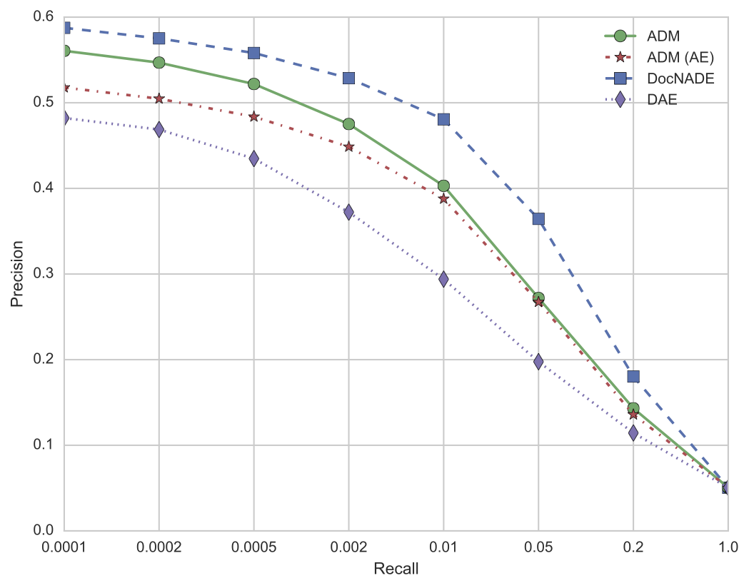
To compare with previous published work in this area (LDA, Replicated Softmax, DocNADE) we ran some experiments with this adversarial model on the 20 Newsgroups dataset. It must be stressed that this is a relatively toy dataset by current standards, consisting of a collection of around 19000 postings to 20 different newsgroups. One open question with generative models (and GANs in particular) is what metric do you actually use to evaluate how well they are doing? If the model yields a proper joint probability over the input, a popular choice is to evaluate the likelihood of a held-out test set. Unfortunately this is not an option for GAN models. Instead, as we are only really interested in the usefulness of the learned representation, we also follow previous work and compare how likely similar documents are to have representations that are close together in vector space. Specifically, we create vectors for every document in the dataset. We then use the held-out test set vectors as “queries”, and for each query we find the closest $N$ documents in the training set (by cosine similarity). We then measure what percentage of these retrieved training documents have the same newsgroup label as the query document. We then plot a curve of the retrieval performance for different values of $N$. The results are shown below.

Here we can see a few notable points:
- The model does learn useful representations, but is still not reaching the performance of DocNADE on this task. At lower recall values though it is better than the LDA results on the same task (not shown above, see the Replicated Softmax paper).
- By using a denoising autoencoder as the discriminator, we get a bit of a boost versus just using a standard autoencoder.
- We get quite a large improvement over just training a denoising autoencoder with similar parameters on this dataset.
We also looked at whether the model produced results that were easy to interpret. We note that the autoencoder bottleneck has weights connecting it to every word in the vocabulary, so we looked to see if specific hidden units were strongly connected to groups of words that could be interpreted as newsgroup topics. Interestingly we find some evidence of this as shown in the table below, where we present the words most strongly associated with three of these hidden units. They do generally fit into understandable topic categories, with a few of exceptions. However, we note that these are cherry-picked examples, and that overall the weights for a specific hidden unit do not tend to strongly associate with single topics.
| Computing | Sports | Religion |
|---|---|---|
| windows | hockey | christians |
| pc | season | windows |
| modem | players | atheists |
| scsi | baseball | waco |
| quadra | rangers | batf |
| floppy | braves | christ |
| xlib | leafs | heart |
| vga | sale | arguments |
| xterm | handgun | bike |
| shipping | bike | rangers |
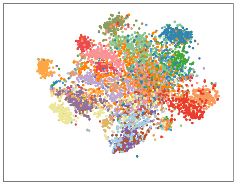
We can also see reasonable clustering of many of the topics in a TSNE plot of the test-set vectors (1 colour per topic), although some are clearly still being confused:

Conclusion
I showed some interesting first steps in using GANs to model documents, admittedly perhaps asking more questions than I answered. In the time since the completion of this work, there have been numerous proposals to improve GAN training (such as this, this and this), so it would be interesting to see if any of the recent advances help with this task. And of course, we still need to see if this approach can be scaled up to larger datasets and vocabularies. The full source code is now available on Github, I look forward to seeing what people do with it.